Joseph M. Knight

The Maze of JCMB - A Network Approach

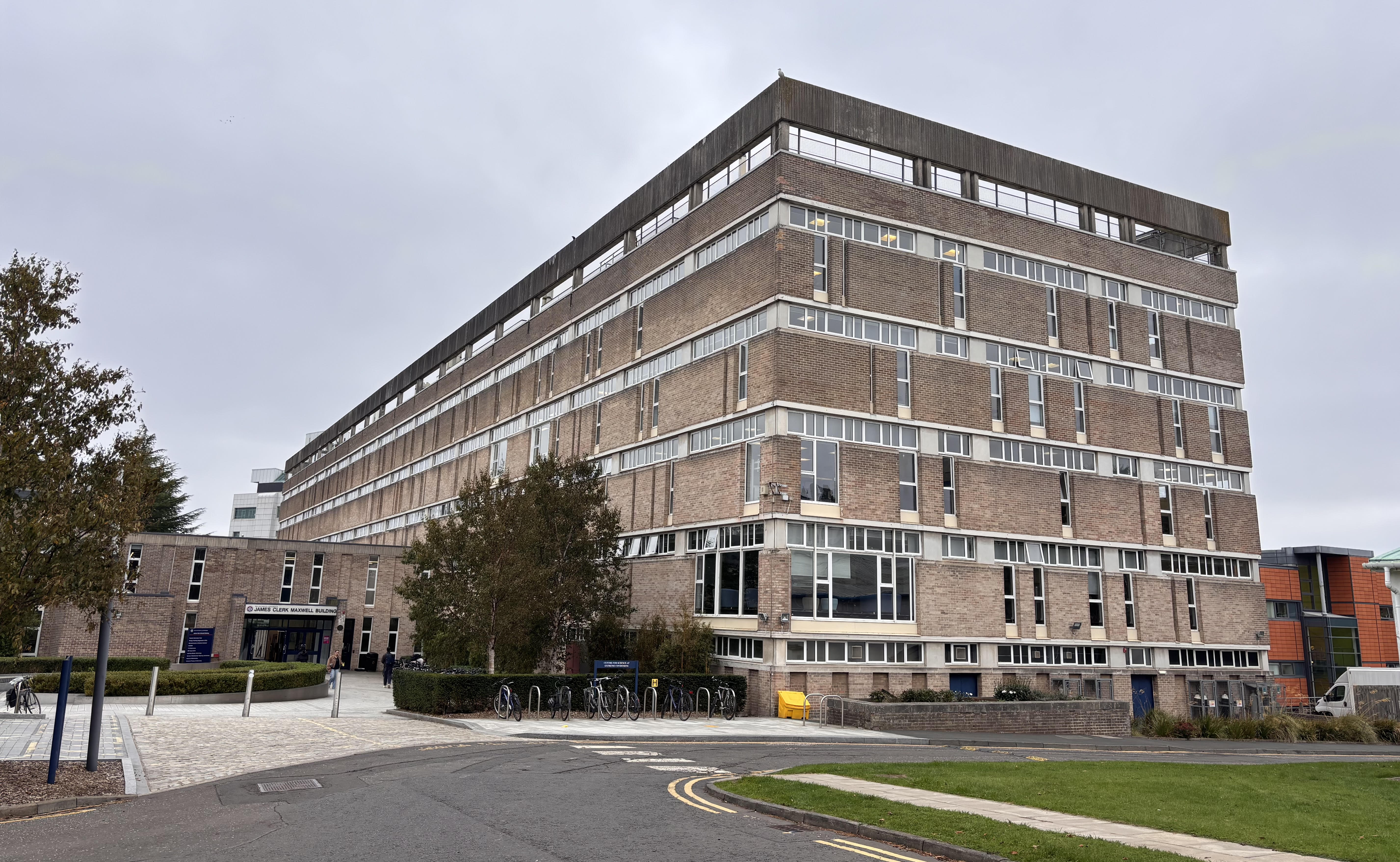
The James Clerk Maxwell Building (JCMB) is home to the School of Physics & Astronomy at the University of Edinburgh. One of the most frequent comments from staff and students (old and new) is that JCMB is a 'maze', with seemingly illogical dead-end corridors and multiple staircase options for traversing floors.

As my research is primarily focused on understanding the network structure of biological systems (See Research), I wondered if it would be possible to apply a similar network approach to better understand the connectivity (or topology) of the building and, ultimately, build a route finding applet to find the shortest path between rooms. On this page I will detail this process and some findings.

JCMB as a Network: Implementation

An introduction to network theory

At the heart of network science is the idea that a physical network can be represented as a mathematical object known as a graph. A given graph \( G\) is defined in terms of a relation betweeen a set of nodes and edges. So, the graph \( G=(V,L) \) is defined in terms of a set \( V \) of \(N \) nodes alongside a set \( L \) of \(E \) edges that connect these nodes.

The most fundemental way of representing our graph \( G\) is through an adjacency matrix \( a_{ij}\). The entries of this matrix tell us whether there exists a connection between two nodes specified by the indices \( i\) and \( j\) such that we have \[ a_{ij}= \begin{cases} 1, \text{if} \; i \;\text{and}\; j \;\text{are connected} \\ 0 \; \text{otherwise} \end{cases} \] For an undirected graph, this adjacency matrix is symmetric (that is, \( a_{ij}=a_{ji}\)) such that the edges encode no directional information. The adjacency matrix that we have introduced above is also implicitly an unweighted graph, that is, it encodes no length information in the edges, only whether they exist or not. Rather than this purely topological representation, we can easily incorporate edge length information using a weighted graph where now our weighted adjacency matrix \(A_{ij} \) has entries given by the length of the edge between nodes \( i\) and \( j\), with the entry still being zero if no such edge exists.

Network Properties

An important property of any given node (especially when it comes to our representation of a building as a network) is the degree of a node. The node degree is defined as the number of neighboring nodes which can be formalised using the unweighted adjacency matrix \( a_{ij}\) as \[ k_i = \sum_j a_{ij} \] In our construction of a JCMB network, nodes of degree one (that is, endpoints) will represent our rooms whilst higher degree nodes, most frequently either degree three or four, will represent junctions in corridors. Interestingly, in the context of spatial networks (networks embedded in physical space rather than more abstract networks such the World Wide Web), the idea of a degree two node is somewhat redundant.

Two interesting network metrics that we will consider look at the global structure of the network. The first of these is the cost \(C\) of the network. This is defined with the weighted adjacency matrix \( A_{ij} \) as \[ C=\frac{1}{2}\sum_{i\neq j} A_{ij}\] which is just a measurement of the total length of edges in the network. A second, more complicated metric that we will introduce is the global efficiency \(E_g\) of the network. This is defined as \[ E_g = \frac{1}{N(N-1)}\sum_{i\neq j}\frac{\ell_{ij}}{d_{ij}}.\] Here, we compare, for each of the \(N(N-1)\) node pairings, the shortest distance \(d_{ij}\) connected the two nodes through the network with the Euclidian straight line distance \(\ell_{ij}\) between the two points. This gives us some measure of the 'transport efficiency' of the network, that is, how easy it is to get from any point on the network to any other point. By normalising these two measures based on the extreme cases of the Minimum Spanning Tree (MST) and Delaunay Triangulation (DT) it is possible to make comparisons of networks across different lengthscales with \(\hat{E}_g\) and \(\hat{C}\).

Building the JCMB Network

The first step in constructing the overall building graph \(G_\text{JCMB}\) is to first build subgraphs \(G_i\) of the individual floors where we have \( i \in [1,7] \cap \mathbb{Z} \). To do this we take the floorplans (which are available here following a WiFi signal strength mapping survey). From each floorplan connectivity trace, we build a spatially embedded network using the sknw package.

With all of the floor subgraphs, we can write the total graph \(G_\text{JCMB}\) in block diagonal form. As shown below, we can then specify the off diagonal staircase 'linker' entries of the weighted adjacency matrix.
\[ G_\text{JCMB} = \begin{pmatrix} \color[rgb]{0.51, 0.714, 0.89}{\begin{pmatrix} & & \\ & G_1 & \\ & & \end{pmatrix}} & \begin{matrix} 0 & 0 & 0 \\ 0 & s^{\color[rgb]{0.51, 0.714, 0.89}{1}\color[rgb]{0, 0, 0}{,}\color[rgb]{0.83, 0.725, 0.541}{2}}_{ij} & 0 \\ 0 & 0 & 0 \end{matrix} & \begin{matrix} 0 & 0 & 0 \\ 0 & 0 & 0 \\ 0 & 0 & 0 \end{matrix} \\[3 mm] \begin{matrix} 0 & 0 & 0 \\ 0 & s^{\color[rgb]{0.51, 0.714, 0.89}{1}\color[rgb]{0, 0, 0}{,}\color[rgb]{0.83, 0.725, 0.541}{2}}_{ij} & 0 \\ 0 & 0 & 0 \end{matrix} & \color[rgb]{0.83, 0.725, 0.541}{\begin{pmatrix} & & \\ & G_2 & \\ & & \end{pmatrix}} & \begin{matrix} 0 & 0 & 0 \\ 0 & s^{\color[rgb]{0.83, 0.725, 0.541}{2}\color[rgb]{0, 0, 0}{,}\color[rgb]{0.84, 0.247, 0.125}{3}}_{ij} & 0 \\ 0 & 0 & 0 \end{matrix} \\[3 mm] \begin{matrix} 0 & 0 & 0 \\ 0 & 0 & 0 \\ 0 & 0 & 0 \end{matrix} & \begin{matrix} 0 & 0 & 0 \\ 0 & s^{\color[rgb]{0.83, 0.725, 0.541}{2}\color[rgb]{0, 0, 0}{,}\color[rgb]{0.84, 0.247, 0.125}{3}}_{ij} & 0 \\ 0 & 0 & 0 \end{matrix} & \color[rgb]{0.84, 0.247, 0.125}{\begin{pmatrix} & & \\ & G_3 & \\ & & \end{pmatrix}} \end{pmatrix} \] The matrix representation above shows the introduction of our staircase (or lift) links between floors, giving us our complete building network.

JCMB Path Finder

Below you can find and interact with the shortest path between rooms in JCMB. The calculation is performed using Dijkstra's algorithm. The 3D plotting employs Plotly. Please note that the Python backend on which this applet requires is hosted by Render. I am using the free tier hosting service which spins down the server with inactvity so opening this page for the first time will lead to a small (~minutes) delay in rendering.